Usage
Below are some simple example uses of the various functions and classes in niteshade. For a more comprehensive overview of niteshade’s functionality, please refer to the API section.
Getting Started
Before we begin, many of the following sections will use various functions and
classes from PyTorch, so let’s go ahead and import PyTorch so we can
focus exclusively on niteshade imports from here on out:
>>> import torch
>>> import torch.nn as nn
Note that in many examples we use torch.randn() to generate example data
tensors. The dimensions are completely arbitrary.
Setting Up an Online Data Pipeline
niteshade makes setting up an online data pipeline easy, thanks to its bespoke
data loader class specifically designed for online learning
niteshade.data.DataLoader.
>>> from niteshade.data import DataLoader
A DataLoader may be instantiated with a particular set of features (X) and
labels (y):
>>> X = torch.randn(100, 3, 32, 32)
>>> y = torch.randn(100)
>>> pipeline = DataLoader(X, y, batch_size=8, shuffle=True)
Alternatively, data may be added by calling the .add_to_cache() method:
>>> X_more = torch.randn(50, 3, 32, 32)
>>> y_more = torch.randn(50)
>>> pipeline.add_to_cache(X_more, y_more)
DataLoader instances have a cache and queue attribute, which together help
ensure that data is batched and loaded consistently. When data is added to a
DataLoader, either during instantiation or by calling the
.add_to_cache() method, it is added to the cache then automatically grouped
into batches of the provided batch size and moved to the queue. Any remaining
points which do not “fit” into a batch are kept in the cache, where they remain
until enough new datapoints are added to form a complete batch. E.g. in the
above case, a total of 150 datapoints have been added to a DataLoader with
a batch size of 8. This results in 18 batches of 8 datapoints (144 datapoints
total) in the queue and 6 points in the cache.
>>> len(pipeline)
18
DataLoader instances are iterators; the queue can be iterated over and
depleted in a for loop:
>>> for batch in pipeline:
...     pass
...
>>> len(pipeline)
0
Note that after executing the above for loop there would still be 6 points in the cache. If we add 2 additional points to the cache we can form a complete batch of 8 which will be added to the queue.
>>> X_last = torch.randn(2, 3, 32, 32)
>>> y_last = torch.randn(2)
>>> pipeline.add_to_cache(X_last, y_last)
>>> len(pipeline)
1
The cache is now empty.
Managing Pipeline Asynchronicity
In many scenarios, data generation and learning are asynchronous. For example,
if data is generated in batches of 10 datapoints (let’s call these episodes for
notational clarity), but the model wants to learn on batches of size 16, then
the model will only be able to do an incremental learning step every 1.6
episodes on average. To complicate matters, if we add deploy a poisoning attack
and implement a defence strategy that rejects suspicious datapoints, the
pipeline becomes even more asynchronous (episodes may now consist of fewer than
16 datapoints if the defence strategy rejects points). To address this
asynchronicity, niteshade workflows generally involve separate generation and
learning loops, each with their own DataLoader (leveraging the cache and
queue to ensure consistent episode and batch sizes). Below is a very simple
example (model, attack and defence strategies not specified):
from niteshade.data import DataLoader

X = torch.randn(100, 5)
y = torch.randn(100)

episodes = DataLoader(X, y, batch_size=10)
batches = DataLoader(batch_size=16)

for epiosde in episodes:

    # Attack strategy deployed (may change shape of episode)
    ...

    # Defense strategy deployed (may change shape of episode)
    ...

    batches.add_to_cache(episode)

    for batch in batches:

        # Incremental learning update
        ...
Note that the inner loop (learning loop) will only execute if the batch
DataLoader contains sufficient datapoints to form a complete batch.
Otherwise, its queue attribute will be empty and iterating over it will do
nothing.
Setting Up a Victim Model
Setting up a victim model (an online learning model which will be the subject
of a data poisoning attack) can be done in two different ways. The simplest way
is to use one of niteshade’s out-of-the-box model classes, e.g.
shade.models.IrisClassifier (designed specifically for the Iris dataset),
shade.models.MNISTClassifier (designed specifically for MNIST), or
shade.models.CifarClassifier (designed specifically for CIFAR-10), for
example:
>>> from niteshade.models import IrisClassifier
>>> model = IrisClassifier(optimizer="adam", loss_func="cross_entropy", lr=1e-3)
However, most users will prefer to create a custom model class. Custom model
classes can be easily created by inheriting the niteshade.models.BaseModel
superclass, providing it the necessary arguments in the constructor, and
filling in the .forward(), and .evaluate() methods. Below is an example
of a simple multi-layer perceptron regressor:
class MLPRegressor(BaseModel):
    """ Simple MLP regressor class. """

    def __init__(self, optimizer="adam", loss_func="mse", lr=1e-3):
        """ Specify architecture, optimizer, loss and learning rate. """
        architecture = [nn.Linear(4, 16), nn.ReLU(), nn.Linear(16, 1)]
        super().__init__(architecture, optimizer, loss_func, lr)

    def forward(self, x):
        """ Execute the forward pass. """
        return self.network(x)

    def evaluate(self, X_test, y_test):
        """ Evaluate the model predictions. """
        self.eval()
        with torch.no_grad():
            y_pred = self.forward(X_test)
            accuracy = 1 - (y_pred - y_test).square().mean().sqrt()
        return accuracy
In the constructor (.__init__() method), the model architecture must be
defined as a list of PyTorch building blocks (layers, activations etc.), then
passed to the BaseModel superclass along with the desired optimiser, loss
function and learning rate (see API section for possible values). The
BaseModel class has a .device attribute which is automatically set to
“cuda” or “cpu” depending on whether a GPU is available, and a .network
attribute which assembles the provided architecture as a callable that passes
inputs through the layers and activations in sequence. Both these attributes
are used in the .forward() method, which implements the forward pass.
Finally, the .evaluate() method computes whichever performance metric we
are interested in analysing during the simulation (accuracy, in this case).
All niteshade models (out-of-the-box and custom) perform incremental learning
updates using the .step() method, which is inherited from BaseModel.
Defining an Attack Strategy
niteshade’s attack module (niteshade.attack) includes several
out-of-the-box classes based on some of the most commonly encountered data
poisoning attack strategies, e.g. LabelFlipperAttacker (which as the name
suggests, flips training labels) and AddLabelledPointsAttacker (which
injects fake datapoints into the learning pipeline).
>>> from niteshade.attack import AddLabelledPointsAttacker
>>> attacker = AddLabeledPointsAttacker(aggressiveness=0.5, label=1)
An attack can be deployed against a batch of datapoints by calling the
.attack() method:
>>> X = torch.randn(10, 5)
>>> y = torch.randn(10)
>>> X_attacked, y_attacked = attacker.attack(X, y)
Custom attack strategies may also be defined following niteshade’s attack class
hierarchy by inheriting from the relevant superclass and filling in the
.attack() method. At the top of the hierarchy is the Attacker class,
which is a general abstract base class for all attack strategies. The next tier
in the hierarchy is comprised of general categories of attack strategies,
namely AddPointsAttacker (for strategies which involve injecting fake
datapoints into the learning pipeline), PerturbPointsAttacker (for
strategies which involve perturbing real datapoints in the learning pipeline)
and ChangeLabelAttacker (for strategies which involve altering training
data labels). Below is an example of a very simple custom attack strategy which
involves appending zeros to the end of training batches:
from niteshade.attack import AddPointsAttacker

class AppendZerosAttacker(AddPointsAttacker):
    """ Append zeros attack strategy class. """

    def __init__(self, aggressiveness):
        """ Set the aggressiveness. """
        super().__init__(aggressiveness)

    def attack(self, X, y):
        """ Define the attack strategy. """
        num_to_add = super().num_pts_to_add(X)
        X_fake = torch.zeros(num_to_add, *X.shape[1:])
        y_fake = torch.zeros(num_to_add, *y.shape[1:])
        return (torch.cat((X, X_fake)), torch.cat((y, y_fake)))
This simple (and ineffective) strategy involves injecting fake datapoints, so
the class inherits from AddPointsAttacker in its constructor. The
aggressiveness attribute is a float between 0.0-1.0 which determines
the proportion of points the attacker is allowed to attack (or append, in this
case). The .attack() method defines the attack strategy, which in this case
is very straightforward. The AddPointsAttacker superclass has a method
.num_pts_to_add() which uses aggressiveness to determine the (integer)
number of points to add. Note that if the attack strategy we wish to define
doesn’t fit into any of the aforementioned categories, we can simply inherit
from Attacker.
Defining a Defence Strategy
Similarly to the attack module, niteshade’s defence module
(niteshade.defence) includes several out-of-the-box classes based on some
of the most well-known defence strategies against data poisoning attacks, e.g.
FeasibleSetDefender (which functions as an outlier detector based on a
“clean” set of feasible points), KNN_Defender (which adjusts labels based
on the consensus of neighbouring points) and SoftmaxDefender (which rejects
points based on a softmax threshold).
>>> from niteshade.defence import SoftmaxDefender
>>> defender = SoftmaxDefender(threshold=0.1)
After an attack has been deployed on a batch of datapoints, a defence can be
implemented to minimise the damage by calling the .defend() method:
>>> X_attacked = torch.randn(10, 5)
>>> y_attacked = torch.randn(10)
>>> X_defended, y_defended = defender.defend(X_attacked, y_attacked)
Custom defence strategies may also be defined following niteshade’s defence
class hierarchy by inheriting from the relevant superclass and filling in the
.defend() method. At the top of the hierarchy is the Defender class,
which is a general abstract base class for all defence strategies. The next
tier in the hierarchy is comprised of general categories of defence strategies,
namely OutlierDefender (for strategies which involve filtering outliers),
ModelDefender (for strategies which require access to the model and its
parameters) and PointModifierDefender (for strategies which modify
datapoints). Below is an example of a very simple custom defence strategy which
involves removing points which have even-valued labels:
from niteshade.defence import Defender

class EvenLabelDefender(Defender):
    """ Even-valued label filtering defence strategy. """

    def __init__(self):
        """ Constructor. """
        super().__init__()

    def defend(self, X, y):
        """ Define the defence strategy. """
        return (X[y % 2 != 0], y[y % 2 != 0])
Although this simple (and ineffective) strategy resembles an
OutlierDefender-type strategy, it doesn’t require a clean feasible set for
outlier detection, and thus we have just inherited from Defender.
Running a Simulation
Once a model has been set up and attack and defence strategies have been
defined, simulating an attack against online learning is very straightforward.
niteshade’s simulation module (niteshade.simulation) contains a
Simulator class which sets up and executes the adversarial online learning
pipeline (the asynchronous double-loop pipeline shown previously):
>>> from niteshade.models import MNISTClassifier
>>> from niteshade.attack import LabelFlipperAttacker
>>> from niteshade.defence import KNN_Defender
>>> from niteshade.simulation import Simulator
>>> from niteshade.utils import train_test_MNIST
>>>
>>> X_train, y_train, X_test, y_test = train_test_MNIST()
>>> model = MNISTClassifier()
>>> attacker = LabelFlipperAttacker(aggressiveness=1, label_flips_dict={1:9, 9:1})
>>> defender = KNN_Defender(X_train, y_train, nearest_neighbours=3, confidence_threshold=0.5)
>>> batch_size = 128
>>> num_eps = 50
>>> simulator = Simulator(X_train, y_train, model, attacker, defender, batch_size, num_eps)
In the above example, we are simulating a digit classification model trained on
MNIST subject to a label-flipping attack (specifically one which flips 1’s and
9’s with 100% aggressiveness) with a k-nearest neighbours defence (k=3, 50%
consensus). We use a helper function from niteshade.utils to load in the
MNIST dataset and specify that the online data pipeline should split the
dataset into 50 sequential episodes. Finally, we set the training batch size to
128 and pass all the above information to the Simulator class before
running the simulation by calling the .run() method:
>>> simulator.run()
The Simulator class has a .results attribute which stores snapshots of
the model’s state dictionary at each episode as well as datapoint tracking
information to monitor the effects of the attack and defence strategies.
Note that the attacker and defender arguments in Simulator are optional and
default to None; simulations can be run without any attack or defence strategy
in place, with just an attack strategy, with just a defence strategy or with
both. If custom model, attack or defence classes have been created, they can be
passed as arguments to the Simulator class exactly as shown above.
Postprocessing Results
niteshade’s postprocessing module (niteshade.postprocessing) contains
several useful tools for analysing and visualising results. Once a simulation
has been run, (by calling Simulator.run(), which populates the .results
attribute), it may be passed to the PostProcessor class in a dictionary
keyed by the name of the simulation. Building off the previous example:
>>> from niteshade.models import MNISTClassifier
>>> from niteshade.attack import LabelFlipperAttacker
>>> from niteshade.defence import KNN_Defender
>>> from niteshade.simulation import Simulator
>>> from niteshade.postprocessing import PostProcessor
>>> from niteshade.utils import train_test_MNIST
>>>
>>> X_train, y_train, X_test, y_test = train_test_MNIST()
>>> model = MNISTClassifier()
>>> attacker = LabelFlipperAttacker(1, {1:9, 9:1})
>>> defender = KNN_Defender(X_train, y_train, 3, 0.5)
>>> batch_size = 128
>>> num_eps = 50
>>> simulator = Simulator(X_train, y_train, model, attacker, defender, batch_size, num_eps)
>>> simulation.run()
>>> simulation_dict = {"example_name": simulation}
>>> postprocessor = PostProcessor(simulation_dict)
We can also run multiple simulations and pass them to PostProcessor:
>>> model1 = MNISTClassifier()
>>> model2 = MNISTClassifier()
>>> model3 = MNISTClassifier()
>>> s1 = Simulator(X_train, y_train, model1, None, None, batch_size, num_eps)
>>> s2 = Simulator(X_train, y_train, model2, attacker, None, batch_size, num_eps)
>>> s3 = Simulator(X_train, y_train, model3, attacker, defender, batch_size, num_eps)
>>> s1.run()
>>> s2.run()
>>> s3.run()
>>> simulation_dict = {"baseline": s1, "attack": s2, "attack_and_defence": s3}
>>> postprocessor = PostProcessor(simulation_dict)
This is useful because the impact of an attack or defence strategy is usually relative to some baseline case. For example, it may be of interest to compare the attacked and un-attacked learning scenarios to isolate the effect of the attack. Similarly, comparing the scenario in which both attack and defence strategies are implemented to the case in which only the attack strategy is implemented can isolate the effect of the defence. Notice that we create 3 separate model instances as we want the models to be independent between the simulations.
PostProcessor can then be used to compute and plot the model’s performance
over the course of the simulation:
>>> metrics = postprocessor.compute_online_learning_metrics(X_test, y_test)
>>> postprocessor.plot_online_learning_metrics(metrics, show_plot=True)
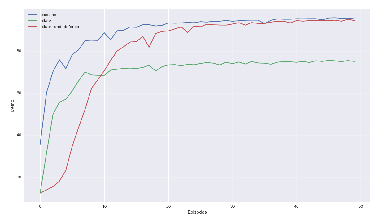
The performance metric that PostProcessor computes and plots on the y-axis
is whatever is written in the model’s .evaluate() method (predictive
accuracy for MNISTClassifier). We can see that in the baseline case, the
model achieves a predictive accuracy across all classes of ~0.95 after 50
episodes. When the model is subjected to the label-flipping attack, it is only
able to achieve a predictive accuracy of ~0.75 (specific accuracy for 1’s and
9’s is likely be even lower). When the kNN defence strategy is deployed against
the label-flipping attack, the model learns more slowly but is able to achieve
a final predictive accuracy of ~0.95 again, meaning the defence strategy is
very effective against this particular attack.
PostProcessor also has a .get_data_modifications() method which
creates a table (pandas DataFrame object) which summarises the simulation
outcomes in terms of the numbers of datapoints which have been poisoned and
defended:
>>> data_modifications = postprocessor.get_data_modifications()
>>> print(data_modifications)
                       baseline  attack  attack_and_defence
poisoned                      0   12691               12691
not_poisoned              60000   47309               47309
correctly_defended            0       0               12677
incorrectly_defended          0       0                 916
original_points_total     60000   60000               60000
training_points_total     60000   60000               60000
In the above table,
poisoned: datapoints perturbed or injected by the attacker
not_poisoned: datapoints not perturbed or injected by the attacker
correctly_defended: poisoned points correctly removed or modified by the defender
incorrectly_defended: clean datapoints incorrectly removed or modified by the defender
original_points_total: total datapoints in the original training dataset
training_points_total: datapoints the model actually gets to train on (certain attack/defence strategies remove datapoints from the learning pipeline)
niteshade.postprocessing also contains a PDF class, which can generate
a summary report of the simulation(s). Adding tables and figures to the report
is easy, as shown below. In this case, our summary report will contain a single
table and plot (the one shown above). If we generated additional plots and
saved them to the /outputs directory, they would also be included in the
report.
>>> from niteshade.postprocessing import PDF
>>> header_title = f"Example Report"
>>> pdf = PDF()
>>> pdf.set_title(header_title)
>>> pdf.add_table(data_modifications, "Datapoint Summary")
>>> pdf.add_all_charts_from_directory("output")
>>> pdf.output("example_report.pdf", "F")
Here, we have saved the report to our current working directory:
$ export REPORT=example_report.pdf
$ test -f $REPORT && echo "$REPORT exists :)"
example_report.pdf exists :)
End-To-End Example
To wrap thing up, here is an end-to-end example of a niteshade workflow using out-of-the-box model, attack and defence classes:
# Imports & dependencies
from niteshade.models import MNISTClassifier
from niteshade.attack import LabelFlipperAttacker
from niteshade.defence import KNN_Defender
from niteshade.simulation import Simulator
from niteshade.postprocessing import PostProcessor, PDF
from niteshade.utils import train_test_MNIST

# Get MNIST training and test datasets
X_train, y_train, X_test, y_test = train_test_MNIST()

# Instantiate out-of-the-box MNIST classifiers
model1 = MNISTClassifier()
model2 = MNISTClassifier()
model3 = MNISTClassifier()

# Specify attack and defence strategies
attacker = LabelFlipperAttacker(aggressiveness=1, label_flips_dict={1:9, 9:1})
defender = KNN_Defender(X_train, y_train, nearest_neighbours=3, confidence_threshold=0.5)

# Set batch size and number of episodes
batch_size = 128
num_eps = 50

# Instatiate simulations
s1 = Simulator(X_train, y_train, model1, None, None, batch_size, num_eps)
s2 = Simulator(X_train, y_train, model2, attacker, None, batch_size, num_eps)
s3 = Simulator(X_train, y_train, model3, attacker, defender, batch_size, num_eps)

# Run simulations (may take a few minutes)
s1.run()
s2.run()
s3.run()

# Postprocess simulation results
simulation_dict = {"baseline": s1, "attack": s2, "attack_and_defence": s3}
postprocessor = PostProcessor(simulation_dict)
metrics = postprocessor.compute_online_learning_metrics(X_test, y_test)
data_modifications = postprocessor.get_data_modifications()
postprocessor.plot_online_learning_metrics(metrics, show_plot=False, save=True)

# Create summary report
header_title = f"Example Report"
pdf = PDF()
pdf.set_title(header_title)
pdf.add_table(data_modifications, "Datapoint Summary")
pdf.add_all_charts_from_directory("output")
pdf.output("example_report.pdf", "F")
This is a relatively simple workflow. For advanced users desiring more customised workflows, consider the following options:
Writing custom model, attack and defence classes following niteshade’s class hierarchy
Writing custom online learning pipelines using
DataLoader’s rather than usingSimulationWriting custom postprocessing functions and plots for the
.resultsdictionary